Map data·5 min read
Core Based Statistical Area: 935 Metro and Micro Areas, Explained
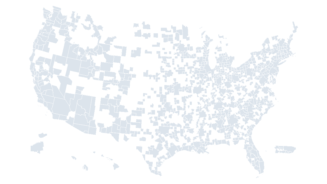
A core based statistical area is one or more whole counties tied to an urban core, and there are 935 of them in the boundary file this site draws from. The number matters because most labor, wage and retail data is published at that level, and none of it joins to a state.
The short answer: 935 areas, two thresholds
A core based statistical area is a county, or a group of counties, that contains a dense urban core and is tied to it by commuting. That is the whole definition, and it explains the two things people trip over: why the count is 935 rather than the 392 metros they remember from a news article, and why the boundary never lines up with a city limit.
The 935 splits into 393 metropolitan areas and 542 micropolitan areas. Open the boundary file and every one of those 935 is present as a separate polygon carrying a five-digit code, which is what a spreadsheet of metro-level figures expects to see in its join column.
Metro and micro are the same object with different thresholds
Both kinds are built the same way and differ only in how large the urban core has to be.
| LSAD | Kind | Core requirement | Areas |
|---|---|---|---|
M1 | Metropolitan statistical area | Urban core of 50,000 or more | 393 |
M2 | Micropolitan statistical area | Urban core of 10,000 to 49,999 | 542 |
| Total | 935 |
The LSAD field is how you tell them apart in the file, and it is worth filtering on rather than trusting the name: a micropolitan area reads exactly like a metropolitan one, Ottumwa, IA versus Dubuque, IA, with nothing in the string to separate them. If your slide claims to show "metros" and you filled all 935, you have quietly included 542 places that no one would call a metro.
Micro areas are not a rounding error in the dataset, either. They are 58% of the shapes, and the largest of them, Elko, NV at 55,293 km², is bigger than every metro except two.
Built from whole counties, so it inherits the gaps
A metro area is not a city with a radius. It is a set of whole counties, which is why it can be drawn with county lines and why the shapes on the map look chunky rather than organic.
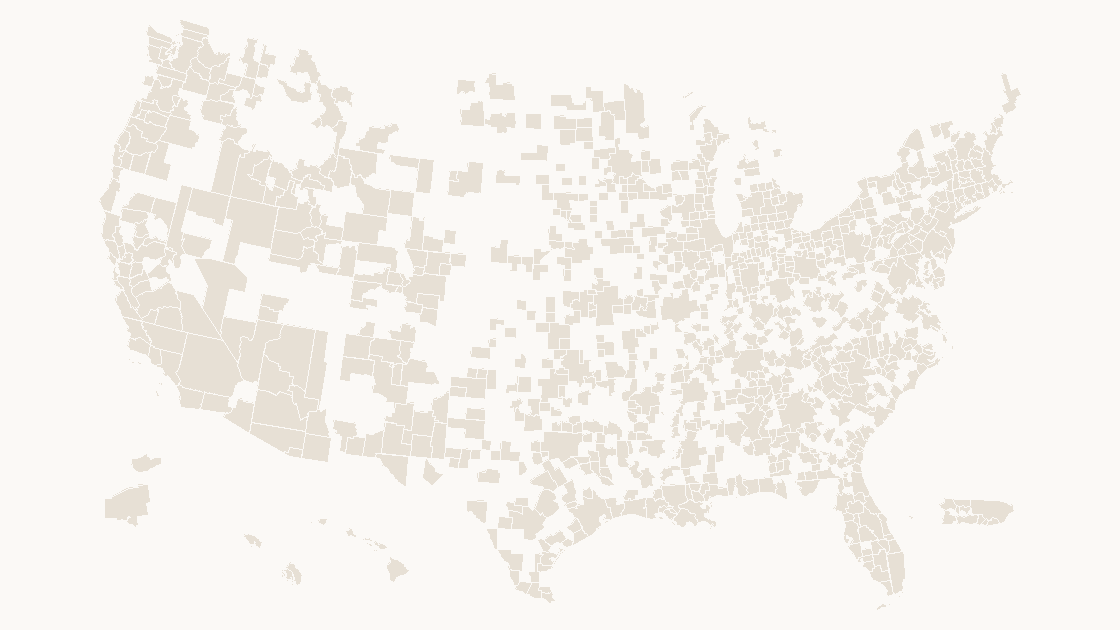
That construction has a consequence the deck makes visible: the areas do not tile the country. Sum the land area of the 935 and you get 4,465,057 km², against 9,162,495 km² for all 3,235 counties in the same release. The metro layer covers 48.7% of the land.
| Measure | Metro and micro areas | Counties |
|---|---|---|
| Features | 935 | 3,235 |
| Land area | 4,465,057 km² | 9,162,495 km² |
| Median feature | 2,540 km² | 1,561 km² |
| Share of county land | 48.7% | 100% |
The median area is 2,540 km², so a typical one holds roughly three and a half counties. Turn that around and the practical warning writes itself: if your figures are metro-level and your template is a county map, about half the country has no value to receive, and it will look like a rendering bug rather than a coverage fact.
Fifty-nine cross a state line, ten are not in a state at all
State lines do not stop a labor market, so the areas cross them. Fifty-nine of the 935 carry a second state code after the comma:
St. Louis, MO-ILBoston-Cambridge-Newton, MA-NHVirginia Beach-Chesapeake-Norfolk, VA-NCWashington-Arlington-Alexandria, DC-VA-MD-WV, which is four jurisdictions in one area
This breaks a specific habit: totalling the areas of a state and comparing the result with the state's own published total. The Missouri side of St. Louis is inside an area that is partly in Illinois, so any state-level sum assembled from metro rows is either double-counted or short, depending on which side you credited.
Ten of the 935 are in Puerto Rico and end in , PR: Aguadilla, Arecibo, Coamo, Coco, Guayama, Lares, Mayagüez, Ponce, San Juan-Bayamón-Caguas and Utuado. They are territories of the United States in the statistical sense and not states in any sense, so a national map either shows them or declares in the footnote that it does not.
Where the shapes are tiny, and where they are enormous
Area varies by three orders of magnitude, and the extremes are worth knowing before you set a label size or a minimum shape width.
| Area | Type | Land |
|---|---|---|
Riverside-San Bernardino-Ontario, CA | Metro | 70,648 km² |
Anchorage, AK | Metro | 68,411 km² |
Elko, NV | Micro | 55,293 km² |
Coco, PR | Micro | 179 km² |
Lares, PR | Micro | 159 km² |
Nantucket, MA | Micro | 119 km² |
Nantucket is a single island county and the smallest thing in the file, and Riverside is 594 times its size. The smallest metropolitan area is Guayama, PR at 328 km², one two-hundredth of Riverside; the next metro up, Carson City, NV, is 374 km².
Fifty-two of the 935 are multipolygons rather than single polygons, because islands and detached coastal pieces are carried as one feature with many parts. That is the right shape for a boundary file, and it is why the metro deck puts 935 selectable shapes on one slide rather than a few thousand fragments.
The five-digit code that is not the one you joined on
Both layers use a five-digit GEOID, and they mean completely different things. A county GEOID is two digits of state plus three of county, so 06037 is Los Angeles County. A CBSA code is a single five-digit number assigned to the area, so 31080 is the Los Angeles metro.
The width matches, the column name matches, and the county file has no CBSA field at all, so nothing in either file stops you from joining one to the other. In this release the two sets have zero values in common, which is the quiet outcome: every row of the join returns a blank, the map shades nothing, and no error is raised anywhere.
The correct join needs a third table, the county-to-CBSA crosswalk, which lists each county GEOID against its CBSA code. Keep it as a separate sheet, never overwrite the boundary files with it, and the same discipline that the FIPS and GEOID walkthrough sets out applies here: the code identifies the row, the name does not.
Choosing between the metro map and the county map
Work backwards from the column you actually have.
| What the data is | Layer | Shapes |
|---|---|---|
| Metro or micro area name, or a five-digit CBSA code | Metro and micro areas | 935 |
| County name or county FIPS | Counties | 3,235 |
| State total | States | 56 |
| Congressional district | Districts, 119th Congress | 441 |
Two habits make the difference between a defensible slide and a confusing one. First, decide what the counties outside the 935 should be: leave them white and note it, or fill them as a single "no metro area" class. Second, do not average metro rates into a county rate. A metro rate is a weighted aggregate of its counties, so the reverse operation is not a plain mean — recompute the numerator and denominator over the counties you want, or use the county table directly.
With 935 shapes, shading is a mechanical step: put the code in one column, the value in the next, look up the class, then apply it with Shape Format → Shape Fill to a selection rather than one shape at a time. The coloring walkthrough covers the selection mechanics, and the county count is the layer underneath this one.
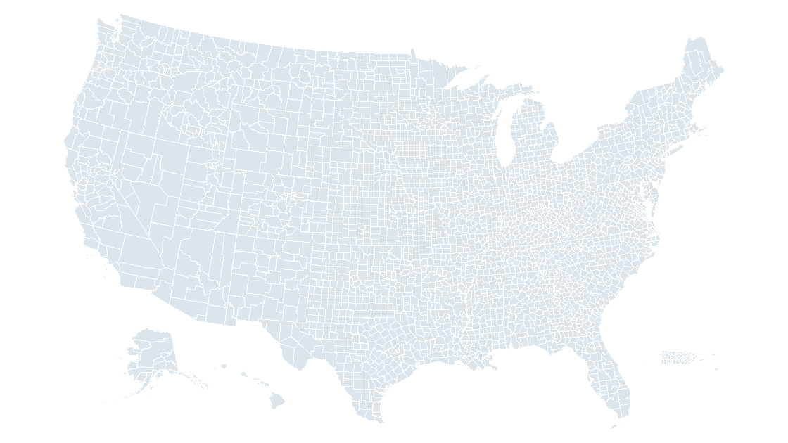
A metro area boundary is not a city boundary and not an urban footprint. If the slide needs to show where people actually live inside the metro, that is a different geography again, and the metro shape will overstate the built-up area by the size of its rural counties.
Check the file before you trust the map
Every number above comes out of two files in this repository, and the check takes a few seconds:
import gzip, json, statistics

raw = open('data/cbsa.geojson', 'rb').read()
cbs = [f['properties'] for f in json.loads(raw)['features']]
cty = [f['properties'] for f in json.load(open('data/county.geojson', encoding='utf-8'))['features']]

metro = [p for p in cbs if p['LSAD'] == 'M1']
micro = [p for p in cbs if p['LSAD'] == 'M2']
land = sum(p['ALAND'] for p in cbs)
print('areas:', len(cbs), 'metro:', len(metro), 'micro:', len(micro))
print('land km2:', land // 10**6, 'county land km2:', sum(p['ALAND'] for p in cty) // 10**6)
print('share of county land: {:.1%}'.format(land / sum(p['ALAND'] for p in cty)))
print('median km2:', statistics.median(p['ALAND'] for p in cbs) // 10**6)
print('smallest:', [(p['NAME'], p['ALAND'] // 10**6) for p in sorted(cbs, key=lambda p: p['ALAND'])[:3]])
print('bytes:', len(raw), 'gzip:', len(gzip.compress(raw, 9)))
areas: 935 metro: 393 micro: 542
land km2: 4465057 county land km2: 9162495
share of county land: 48.7%
median km2: 2540
smallest: [('Nantucket, MA', 119), ('Lares, PR', 159), ('Coco, PR', 179)]
bytes: 2519303 gzip: 881475Two point five megabytes of coordinates, 881 KB compressed, for a layer that answers questions the state map cannot. The 48.7% is the line to remember: it is the reason a metro figure on a county map always leaves half the country blank.
Is a metro area the same as a county?
What separates a metropolitan area from a micropolitan one?
Why does my county map go blank when I shade metro data?
Which column do I join metro data on?
All 935, already drawn
935 metropolitan and micropolitan areas, each an independent named shape carrying its CBSA code, in three themes. $9.99, one-time download.
See the metro areas mapQuestions
Is a metro area the same as a county?
What separates a metropolitan area from a micropolitan one?
Why does my county map go blank when I shade metro data?
Which column do I join metro data on?
Written in-house. Boundary counts are checked against the published files, and every figure on this page can be reproduced from the source named in it.